Mathematica
Vector Functions and Parametric Curves

Parametric, or vector, equations are essential in describing curves in space. This short project will introduce you to some of their properties and applications. Feel free to cut and paste the input code found on this page right into Mathematica just make sure you remember to change the cell style from text to input before you press enter.

Part I. Curves in the plane

A vector is represented in Mathematica simply as a list. For example, a vector pointing in the northeasterly direction of the plane is {1,1}. A vector function is then a list in which each element is a function. For example, the vector function

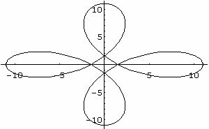
R(t)=(6cost + 5cos3t)i + (6sint-5sin3t)j

may be specified in Mathematica by

R[t_] := {6 Cos[t] + 5 Cos[3 t], 6 Sin[t] - 5 Sin[3 t]} ENTER

To draw the curve described by this vector function, use the command:

ParametricPlot[R[t],{t, 0, 2 Pi}] ENTER

Not bad. You can learn more about the function ParametricPlot by using the on-line help. Simply type ?ParametricPlot to learn the format of the command, and ??ParametricPlot to learn more. In particular, you'll learn the options available to ParametricPlot, one of which is AspectRatio. You may use this option to display the plot using equal scales on the two axes, as follows

ParametricPlot[R[t],{t, 0, 2 Pi}, AspectRatio->Automatic] ENTER

Exercises

1. Draw some more pictures of curves in the plane. The following are all nice looking curves. Be sure to plot them over a range of t which shows the entire curve. Explain how you determined what range of t to use.

a) R(t) = (8 cos t + cos 4t)i + (8 sin t - 2 cos 4t)j ;

b) R(t) = (cos t + 5 cos 3t)i + (6 cos t - 5 sin 3t)j ;

c) R(t) = (3 cos t + cos 3t)i + (2 sin t - sin 2t)j ;

d) R(t) = ( sin ( t/3) , sin ( t/4));

e) R(t) = ( sin ( t/4) , sin (3t/4 ));

f) R(t) = sin 2t i + sin 3t j ;

g) R(t) = t i + 2 t j for 0 <t <2Pi;

h) R(t) = ( sin 2t i + sin 3t j ) + ( t i + 2 t j ) for 0 <t <2Pi.

Comment intelligently on any interesting features you observe in your pictures. Hint: zoom in on interesting featutes of the curves.

2. Explain the differences you see between the plots for parts d and e . Notice that the curve in part h is just the sum of the curves in f and g .

3. Explain the interesting features of the curve in part h .

Part II. Arc length and rolling wheels

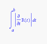
The length of the curve described by the vector function is given by

Let's see how this works; we'll try something for which we already know the answer:

R[t_] := {a Cos[t], a Sin[t]} ENTER
Integrate[Sqrt[R'[t].R'[t]],{t,0, 2 Pi}] ENTER

2 Sqrt[a² ] Pi

Just what we already know about the length of a circle!

If a wheel of radius a rolls along the x -axis without slipping, the path of a point on the rim of the wheel is given by the vector function R(t) = a (t - sin t) i + a(1-cos t)j . This curve is called a cycloid, and is discussed in your calculus book. Let's find the distance the point travels in one revolution:

R[t_] :={t - Sin[t],1 - Cos[t]} ENTER
Integrate[Sqrt[R'[t].R'[t]],{t,0, 2 Pi}] ENTER

Exercises

4. Draw the cycloid R(t) = (t - sin t) i + (1 - cos t ) j .

5. Find a vector equation for the path of a point on the wheel that is at a distance b from the center; and for a = 1, draw the picture of the path for a few values of b. Try values of b larger and smaller than 1.

6. Let d (b) = the distance a point b units from the center of a wheel of radius a = 1 travels in one revolution of the wheel. Draw the graph of d (b) for some appropriate values of b<=1. What are the maximum and the minimum values of d (b)?

7. Use Mathematica to estimate how far from the center of the wheel a point should be in order that the distance it travels in one revolution of the wheel is 90% of the distance traveled by a point on the rim of the wheel.

Part III. Curves in space

The Mathematica function ParametricPlot3D can be used to plot either curves or surfaces in three dimensional space. You can learn about this command by typing ?ParametricPlot3D or ??ParametricPlot3D.

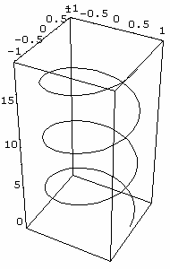
Here's an example in which we plot the helix with parametric equation

R(t) = ( cos t , sin t , t )

ParametricPlot3D[{Cos[t],Sin[t],t},{t,0,6 Pi}] ENTER

This doesn't look too good. Next we use the option BoxRatios to change the shape of the box in which the plot is displayed.

ParametricPlot3D[{Cos[t],Sin[t],t},{t,0,6 Pi}, BoxRatios->{1,1,2}] ENTER

Much better!

Exercises

8. Sketch each of the following curves in three space, as well as three examples of your own choosing. You may wish to experiment with some options such as Boxed, AxesLabel, or use the 3 D ViewPoint Selector (located in the Prepare Input submenu of the Action menu) to set the option ViewPoint. In particular, some of the plots may appear less cluttered if you set Boxed->False. These options are explained in more detail in the project on surfaces.

a) R(t) = cos t i + sin t j + t 2 k,

b) R(t) = ( cos t , sin t , .5 sin ( 4 t ) ),

c) R(t) = sin ( t/4 ) i + sin (3t/4 ) j + sin t k.

Teacups

Index